Report Pivots
Pivot tables are used to view a quick summary and analysis of large amounts of data in lists and tables. Pivot tables are used in excel applications with excel functionalities like drill down functionality into raw data. Data in pivot tables are organized in a tabular layout with each column having a unique name. The layout in which the data should be displayed can be selected from different pivot table styles available.
Creating a Pivot
- Click the Pivots
 icon to open a new tab with the default pivot name Sample Pivot.
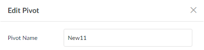
 - Click the
 icon located in the tab name to enter the name of the pivot.
- Click the
 icon to create a new pivot definition. Multiple pivots can be created for a single Report.
- Drag and drop report columns from the left side over to the Pivot sections on the right side to create a pivot.
- Click the
 icon to delete the pivot tab.
 - Reorder the values in all the sections using the
 icons.
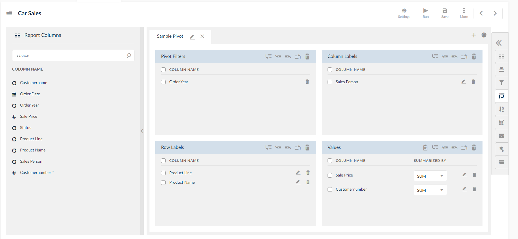
Pivot Panels Explained
Every New Pivot tab has four small sections:
- Pivot Filters
- Column Labels
- Row Labels
- Values
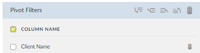
Pivot Filters Section
The pivot filters section consists of the columns that are selected as page filters for the Pivot definition. Drag or use the navigation keys to move the columns to Pivot filters section and use the delete option for single or mass deletion of the filters.
- From each section, delete a column one at a time by clicking the
 icon from a specific section.
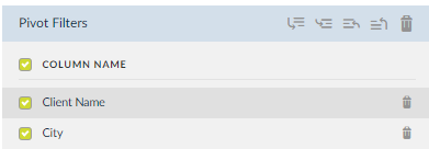
- To delete multiple filters, click the multi-select check box from the top level of each section to check the filters to be deleted and click the
 icon in the top right corner
Columns Section
Drag and drop report columns into the pivot columns sections to reflect those columns in the pivot table output. Like Pivot Filters, entities in the Columns can be moved and/or deleted. Column labels in the Pivot layout can be used in order to display the grouping horizontally.
Row Labels Section
In the Rows section, edit the columns to set subtotals by clicking the ![]() icon. Upon clicking the icon:
icon. Upon clicking the icon:
- A pop up window is displayed with the Source Column, Sub Total and Row Sort fields.
- To select a specific aggregation for Sub Totals instead of automatic, click the
 icon.
icon.
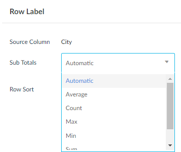
- Select the aggregation function and click OK.
- To exit the edit mode without saving any changes, click Cancel.
Values Section
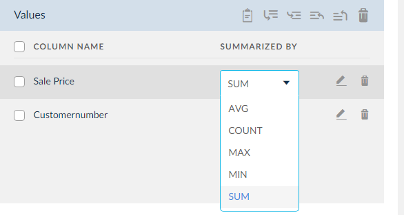
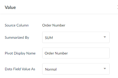
In the Value section, edit the column to set Summarized By, Pivot Display Name and Data Filed Value As by clicking the icon. Upon clicking the edit icon:
- A pop up window will be displayed, where entries in the Summarized By field can be changed by clicking the
 icon and selecting from the drop down.
- The display name of the column on pivot can be changed by overwriting the current name in the field.
- To change Data Field Value As, click the
 icon. There are 3 choices:
- Normal
- % of
- % of Row
Click the desired method.
- To save changes, click OK.
- To exit out of edit mode without saving changes, click Cancel.
Summary Calculations
Add an additional calculation to the columns mentioned in the Values Panel of the Pivot section. The calculated values are available as a part of Excel output.
- Drag and drop the column in the values section.
- Click the
 icon to open the summary calculations window. Click the fx window to enter the calculation column window.
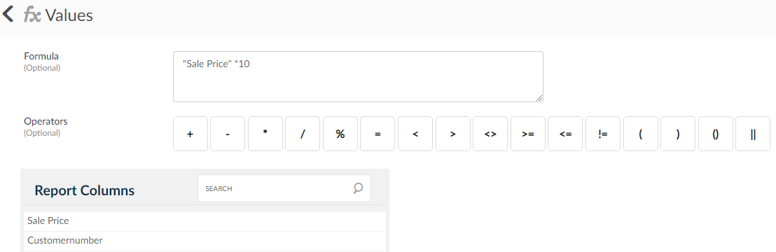
- Drag the column and create the formula and click Save.
- Fill the other-self explanatory options and click Save.
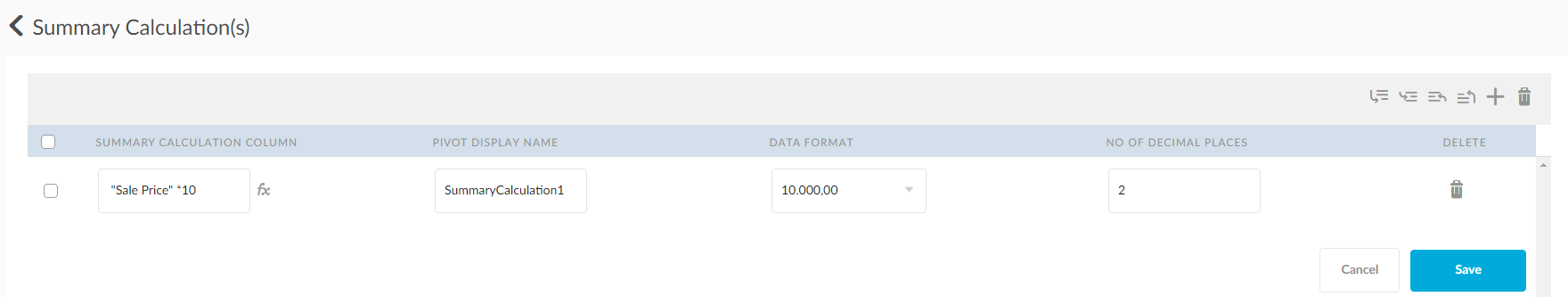
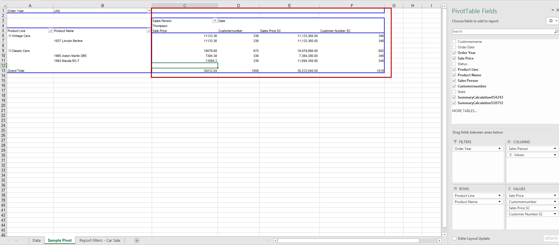
- In Excel output, click the Pivot tab to view the output.
Advanced Settings
Change advanced settings of a pivot by clicking the ![]() icon at the end of the pivot tabs. A pop up window is displayed with options to customize the pivot table.
icon at the end of the pivot tabs. A pop up window is displayed with options to customize the pivot table.
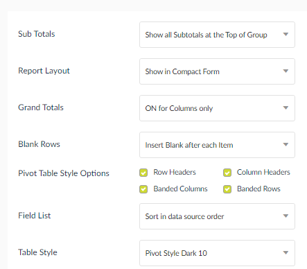
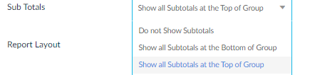
Choose how the Sub Totals should be displayed in the Pivot table by selecting a value in the Sub Totals field. The available options are to display subtotals at the top of the group, bottom of the group or nowhere else. Click the ![]() icon to display choices to choose from.
icon to display choices to choose from.
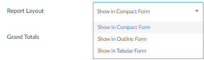
The Report Layout can also be edited in the pivot table. Click the ![]() icon from the Report Layout to view the available choices.
icon from the Report Layout to view the available choices.
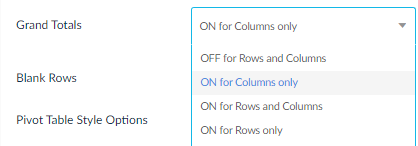
Also choose how the Grand totals should be displayed on the Pivot by selecting a value in the Grand Totals field. cChoose the value from the drop down by clicking ![]() from this field.
from this field.
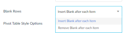
Within the pivot table, separate each group of row data by using the insert method. Click ![]() from the Blank Rows field to insert a blank after each item or remove a blank after each column.
from the Blank Rows field to insert a blank after each item or remove a blank after each column.
In the Pivot Table Style Options, select from Banded Rows, Banded Columns, Column Headers and Row Headers options.
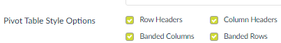
- Banded Rows: This functionality is used to group rows together using color shading for alternate rows. When chosen, every row in the pivot table data will have a shade color.
- Banded Columns: This functionality is used to group columns together. When chosen, every column in the pivot table data will have a shaded color.
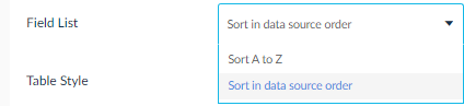
The Field List option allows the user to select the order in which data to be sorted in the Pivot table is present. Click ![]() from the field list box to view the sort options available. The default value for this field is to sort in data source order.
from the field list box to view the sort options available. The default value for this field is to sort in data source order.
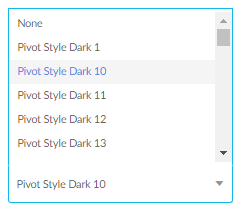
Within the Excel pivot table options lie options for table style. The table style allows the user to select the display style of data within the pivot table. There are different table styles provided by Excel. The style can be chosen during the creation of the pivot or once the report has been downloaded into an Excel output. Click ![]() from the Table Style field to display available table styles.
from the Table Style field to display available table styles.
Once all choices have been selected, click Save. To exit without saving choices, click Cancel.